1D transient diffusion#
Transient diffusion problem is one of the most common phenomenon of real flow problems. Compared to the steady-state diffusion problem, non steady-state diffusion problem need to consider the impact of time derivatives on constant variables.
Problem setup#
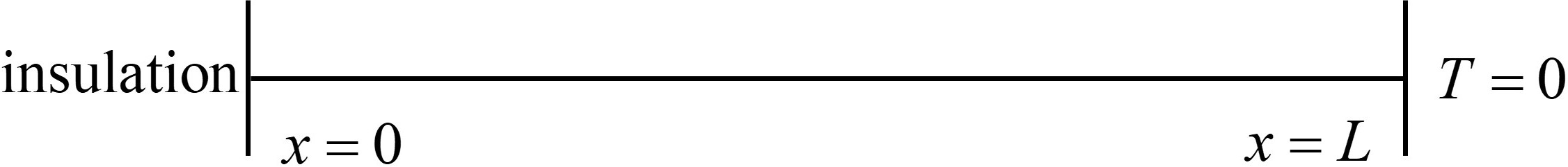
Consider a one-dimensional non steady-state advection problem where a field variable \(\phi\) is transported through the non steady-state diffusion process from \(x = 0\) to \(x = L\) in a one-dimensional domain. All the initial temprature is \( T = 200^\circ C\). At one moment, the the east of the field instantly transforms into \(0^\circ C\), while the west maintains insulation. The fluid volumetric heat capacity(\(\rho c \)) is \(1. 0 \times1 0^{7} \mathrm{~ J / ( m^{3} \cdot~ K ) ~} \), \(L = 0.02\) m, and the thermal conductivity \(k=10\) W/(m \(\cdot\) K). The domain is shown in the figure below.
The mathematical model for one-dimensional non steady-state diffusion problem is $\( \rho c \frac{\partial T}{\partial t} = \frac{\partial}{\partial x} \left( k \frac{\partial T}{\partial x} \right) \)$
The initial conditions are \(T = 200^\circ C (t=0 \text{ s})\). The boundary conditions are $\( \begin{align*} \frac{\partial T}{\partial x} &= 0 \quad && (x=0, t>0 \text{ s}) \\ T &= 0 ^\circ \text{C} \quad && (x=L, t>0 \text{ s}) \end{align*} \)$
The analytical solution for the problem is
where $\( \lambda_n = \frac{(2n-1)\pi}{2L}, \quad \alpha = \frac{k}{\rho c} \)$
Solve problem#
Define grid#
Divide the rod evenly into 5 control volumes, as a result, the length of each control volume becomes \(\Delta x=0.004\) m.
![]()
Discrete the non steady-state advection equation#
The control equation of the 1d non steady-state advection equation is $\(\rho c \; \frac{\partial T} {\partial t}=\frac{\partial} {\partial x} \Big( k \; \frac{\partial T} {\partial x} \Big)+S\)\( where the\)c\(is the specific heat capacity of material and the\)k\(is the material thermal conductivity. Then we integrate the control equation during the \)\Delta t$ in control volumn.
By Gaussian formula, the volume integral can be converted into area fraction.
We deal the time derivatives as $\(\frac{T_{P}-T_{P}^{0}} {\Delta t}\)\( where \)T_{P}^{0}\( is the temperature of \)P\( point at \)t\( and \)T_{P}\( is the temperature of \)P\( point at \)t+\Delta t\(. The left side can be wrote as \)\(\int_{\Delta V} \biggl[ \int_{t}^{t+\Delta t} \rho c \ \frac{\partial\, T} {\partial t} \mathrm{d} t \biggl] \mathrm{d} V \approx\int_{\Delta V} \biggl[ \int_{t}^{t+\Delta t} \rho c \ \frac{T_{P}-T_{P}^{\vee}} {\Delta t} \mathrm{d} t \biggl] \mathrm{d} V=\rho c \left( \, T_{P}-T_{P}^{\vee} \, \right) \Delta V \)\( Eventually, the discreted equation is \)\(\rho c({T_P} - T_P^0)\Delta V = \int_t^{t + \Delta } [ ({k_e}A\;\frac{{{T_E} - {T_P}}}{{\Delta {x_{PE}}}}) - ({k_w}A\;\frac{{{T_P} - {T_W}}}{{\Delta {x_{WP}}}})]dt + \int_t^{t + \Delta t} {\overline S } \Delta Vdt\)$
To calculate the time integral of the diffusion term on the right side of equation above, we need to provide the relationship between the node temperatures \(T_{P}\), \(T_{E}\), and \(T_{W}\) over time, which is unknown. The usual approach is to use the temperature at time \(t\) (such as \(T_{P}^{0}\)) and the temperature at time \(t+\Delta t\) (such as \(T_{P}\)) to weight and combine them to form the average temperature within this time interval, and then integrate and calculate. Mathematically, it manifests as $\(\overline{{{{T_{P}}}}}=\theta T_{P}+( 1-\theta) \ T_{P}^{0} \)\( The time integration is \)\(I_{T}=\int_{t}^{t+\Delta t} T_{P} \, \mathrm{d} t=\left[ \theta T_{P}+\left( 1-\theta\right) T_{P}^{0} \right] \Delta t \)\( Take it into the discreted equation and to be divided by \)A \Delta t$, we can get
Organize it into something familiar to us $\(\begin{aligned} {{a_{P} T_{P}=}} & {{} {{} a_{W} \big[ \theta T_{W}+( 1 \!-\! \theta) \, T_{W}^{0} \big]+a_{E} \big[ \theta T_{E}+( 1 \!-\! \theta) \, T_{E}^{0} \big]+\big[ a_{P}^{0} \!-\! ( 1 \!-\! \theta) a_{W}-( 1 \!-\! \theta) a_{E} \big] T_{P}^{0}+b}} \\ \end{aligned} \)\( where \)\( a_{W}=\frac{k_{w}} {\Delta x_{W P}} \,, \, \, a_{E}=\frac{k_{e}} {\Delta x_{P E}} \,, \, \, a_{P}=a_{P}^{0} \,, \, \, a_{P}^{0}=\rho c \, \, \frac{\Delta x} {\Delta t} \,, b=\bar{S}\Delta x \)\( The choose of \)\theta$ can determine the specific form of the equation, as the table
\(\theta\) |
Description |
|---|---|
0 |
Explicit scheme |
0.5 |
Crank-Niclsion scheme(Implicit) |
1 |
Completely implicit scheme(Implicit) |
Solve the equation by explicit method#
We can linearization the sourse term as $\(b = S_u + S_p T_p^0\)\( and take \)\(\theta = 0\)\( into the equation above. The discreted non steady-state advection equation by explicit method is \)\( a_{P} \, T_{P} \!=\! a_{W} T_{W}^{0} \!+\! a_{E} T_{E}^{0} \!+\! \big[ \, a_{P}^{0} \!-\! ( a_{W} \!+\! a_{E} \!-\! S_{P} ) \, \big] T_{P}^{0} \!+\! S_{u} \)\( , where \)\(a_{W}=\frac{k_{w}} {\Delta x_{W P}} \,, \, \, a_{E}=\frac{k_{e}} {\Delta x_{P E}} \,, \, \, a_{P}=a_{P}^{0} \,, \, \, a_{P}^{0}=\rho c \, \, \frac{\Delta x} {\Delta t} \)$
According to the requirement of boundedness in discrete equations, all coefficients in the equation should be positive values, and the source term should be zero. Therefore we have
$\(a_{P}^{0}-a_{W}-a_{E} > 0. \)\(
and we can solve it as
\)\( \Delta t \leq\rho c \; {\frac{( \Delta x )^{2}} {2 k}} \)\(
, which also means the discrate equation imposes a fairly strict constraint on the maximum value of the calculation time step \)\Delta t $ for explicit formats. This will result in significant costs for improving computational accuracy in actual calculations, as the maximum possible time step decreases as the grid spatial scale decreases (grid refinement). Therefore, the explicit format is not suitable for calculating non-stationary problems in general situations. However, when the time interval is carefully selected to meet the requirements of limit above, the explicit format is still effective for calculating simple diffusion problems.
Here we go!
Internal Nodes 2, 3, 4
The discrete equation satisfied by the internal nodes is
where
Boundary Nodes 1
Under adiabatic conditions, take \(\theta=0\), \(\bar{S} = 0\), \(k_{w}= 0\) into above equation. The control equation for the boundary node 1 is
Boundary Nodes 5
The temperature of east interface node is a constant \(T_{B}\). The control equation for the boundary node 5 is $\( \rho c \Big( \frac{T_{P}-T_{P}^{0}} {\Delta t} \Big) \Delta x=\left[ \frac{k ( T_{B}-T_{P}^{0} )} {\frac{\Delta x} {2}} \right]-\left[ \frac{k ( T_{P}^{0}-T_{W}^{0} )} {\Delta x} \right] \)$
Organize coefficient matrix By organizing the coefficient of above nodes, we can get
node |
\(a_{W}\) |
\(a_{E}\) |
\(a_{P}^{0}\) |
\(a_{P}\) |
\(S_{P}\) |
\(S_{u}\) |
|---|---|---|---|---|---|---|
1 |
0 |
\({\frac{k} {\Delta x}}\) |
\(\rho c {\frac {\Delta x}{\Delta t}}\) |
\(a_{P}^{0}\) |
0 |
0 |
2,3,4 |
\({\frac{k} {\Delta x}}\) |
\({\frac{k} {\Delta x}}\) |
\(\rho c {\frac {\Delta x}{\Delta t}}\) |
\(a_{P}^{0}\) |
0 |
0 |
5 |
\({\frac{k} {\Delta x}}\) |
0 |
\(\rho c {\frac {\Delta x}{\Delta t}}\) |
\(a_{P}^{0}\) |
\(-{\frac{2k} {\Delta x}}\) |
\({\frac{2k} {\Delta x}} T_{B}\) |
Limitation of \(\Delta t\) by explicit method
Solve algebraic equations (explicit method)#
import numpy as np                      # for array operation
from matplotlib import pyplot as plt    # for plotting figures
# -----------------------------------------------------------------------
dt = 2.0                                # time step size(dt<8)
# -----------------------------------------------------------------------
total_time = 120                        # total simulation time
nx = 5                                  # number of spatial grid points
L = 0.02                                # length of the domain
dx = L / nx                             # spatial grid size
x = np.linspace(0.5*dx, L-0.5*dx, nx)   # spatial grid points
T0 = 200                                # initial temperature
rho_c = 1.0e7                           # fluid density plus specific heat
k = 10                                  # thermal conductivity
aW = k/dx
aE = k/dx
ap0 = rho_c * dx / dt
# Calculate numerical solution
def analytical_solution(x, t, k=k, rho_c=rho_c, L=L):
    result = np.zeros_like(x)           # initialize result array
    alpha = k / rho_c
    for i in range(1, 1000):
        lamda_i = (2 * i - 1) * np.pi / (2 * L)
        result += 800 / np.pi * (-1) ** (i + 1)/(2 * i - 1) * np.exp(-alpha * lamda_i**2 * t) * np.cos(lamda_i * x)

    return result
# Renew coefficients
def renew_explicit(a, b, nx):
    for i in range(1, nx + 1):
        a[i][i] = ap0

    b[1] = aE * T_old[2] + (ap0 - (aE + 0 - 0)) * T_old[1]

    for i in range(2, nx):
        b[i] = aW * T_old[i - 1] + aE * T_old[i + 1] + (ap0 - (aW + aE - 0)) * T_old[i]

    b[nx] = aW * T_old[nx - 1] + (ap0 - (aW + 0 + 2 * aW)) * T_old[nx]
# TDMA iteration
def TDMA(a, b, T, nx):
    C = np.zeros(nx + 1)
    phi = np.zeros(nx + 1)
    alph = np.zeros(nx + 1)
    belt = np.zeros(nx + 1)
    D = np.zeros(nx + 1)
    A = np.zeros(nx + 1)
    Cpi = np.zeros(nx + 1)

    for j in range(1, nx + 1):
        belt[j] = -a[j][j - 1]
        D[j] = a[j][j]
        alph[j] = -a[j][j + 1] if j < nx else 0
        C[j] = b[j]

    for j in range(1, nx + 1):
        denom = D[j] - belt[j] * A[j - 1]
        A[j] = alph[j] / denom if denom != 0 else 0
        Cpi[j] = (belt[j] * Cpi[j - 1] + C[j]) / denom if denom != 0 else 0

    phi[nx] = Cpi[nx]
    for j in range(nx - 1, 0,  - 1):
        phi[j] = A[j] * phi[j + 1] + Cpi[j]

    for j in range(1, nx + 1):
        T[j] = phi[j]
# Jacobi iteration
def Jacobi(A,b,T,k):
    AA = A[1 : nx + 1, 1 : nx + 1]
    bb = b[1 : nx + 1]
    n = AA.shape[1]
    D = np.eye(n)
    D[np.arange(n),np.arange(n)] = AA[np.arange(n),np.arange(n)]
    LU = D - AA
    X = np.zeros(n)
    for i in range(k):
        D_inv = np.linalg.inv(D)
        X =  np.dot(np.dot(D_inv,LU),X) + np.dot(D_inv,bb)
    for i in range(1 ,nx + 1):
        T[i] = X[i - 1]
# Output results
def output():
    print("-----------")
    print("time = {}".format(time))
    for i in range(1, nx + 1):
        print(T[i])
# Major routine
a = np.zeros((nx + 1, nx + 1))      # left side of matrix
b = np.zeros(nx + 1)                # right side of matrix
T = np.zeros(nx + 1)                # temperature at current time step
T_old = np.zeros(nx + 1)            # temperature at previous time step
time = 0.0                          # current time

for i in range(1, nx + 1):
    T[i] = T0
    T_old[i] = T0

output_explicit_dt_2 = np.zeros((3, nx))    # to store output for dt=2
maker = 0

# Time loop
while time <= total_time:
    time += dt
    renew_explicit(a, b, nx)                # calculate explicit coefficients
    # TDMA(a, b, T, nx)                     # solve the system of equations using TDMA
    Jacobi(a, b, T, nx)                     # solve the system of equations using Jacobi
    for i in range(1, nx + 1):
        T_old[i] = T[i]                     # update previous temperature values
    output()
    if time % 40 == 0:
        output_explicit_dt_2[maker, :] = T[1:nx + 1]
        maker += 1
-----------
time = 2.0
200.0
200.0
200.0
200.0
150.0
-----------
time = 4.0
200.0
200.0
200.0
193.75
118.75
-----------
time = 6.0
200.0
200.0
199.21875
185.15625
98.4375
-----------
time = 8.0
200.0
199.90234375
197.55859375
176.07421875
84.66796875
-----------
time = 10.0
199.98779296875
199.62158203125
195.166015625
167.333984375
74.9267578125
-----------
time = 12.0
199.9420166015625
199.11041259765625
192.24395751953125
159.2620849609375
67.7459716796875
-----------
time = 14.0
199.83806610107422
198.3560562133789
188.97953033447266
151.94530487060547
62.248992919921875
-----------
time = 16.0
199.6528148651123
197.36924171447754
185.52231788635254
145.36254405975342
57.898783683776855
-----------
time = 18.0
199.36736822128296
196.17382287979126
181.98321163654327
139.44954574108124
54.35705780982971
-----------
time = 20.0
198.9681750535965
194.79918964207172
178.44032980501652
134.12969298660755
51.404354348778725
-----------
time = 22.0
198.4470518771559
193.27545533888042
174.9463576823473
129.32785525918007
48.89393309131265
-----------
time = 24.0
197.80060230987146
191.63076769909821
171.53518208651803
124.97592779109254
46.72469008946791
-----------
time = 26.0
197.0293729835248
189.89004882387235
168.22722350116237
121.01442986531765
44.824922279804014
-----------
time = 28.0
196.13695746356828
188.07461117849016
165.03347746202053
117.39234062160904
43.142380158042215
-----------
time = 30.0
195.12916417793352
186.20226274956622
161.9584770715278
114.06623766871463
41.63803017647752
-----------
time = 32.0
194.0133014993876
184.28765221835735
159.00242035593095
110.99924165753664
40.28204856888778
-----------
time = 34.0
192.79759533925883
182.34270439568283
156.16267700143496
108.15998985875483
39.051185562746944
-----------
time = 36.0
191.49073397131187
180.37706233934887
153.43484453288093
105.52172521458888
37.926989709061196
-----------
time = 38.0
190.1015250173165
178.39849406753578
150.81348184390293
103.06152319118443
36.89458421998686
-----------
time = 40.0
188.63864614859392
176.41324640830425
148.29261354026724
100.75965065137456
35.94180553638984
-----------
time = 42.0
187.1104711810577
174.42634226733585
145.86607228766027
98.59904037311306
35.058584791665474
-----------
time = 44.0
185.5249550668425
172.44182463409166
143.52772704580133
96.56486241475051
34.23649554143006
-----------
time = 46.0
183.88956376274868
170.46295373964924
141.27163116545626
94.64417463446681
33.468417515237604
-----------
time = 48.0
182.21123750986123
168.49236467076256
139.0921144208567
92.82563706093684
32.748282776331855
-----------
time = 50.0
180.4963784049739
166.53219249441165
136.98383603210496
91.09927744535119
32.07088136782452
-----------
time = 52.0
178.75085516615363
164.5841711754436
134.94181076654908
89.45629775900458
31.431710535559223
-----------
time = 54.0
176.98001966731488
162.64971162317056
132.96141669171783
87.88891348201697
30.826856304600092
-----------
time = 56.0
175.18873116179685
160.72996326225703
131.03839065693683
86.39021923605249
30.25289937562718
-----------
time = 58.0
173.3813851743544
158.82586267403448
129.1688158049913
84.95407568110987
29.70683951427355
-----------
time = 60.0
171.56194486181442
156.93817212794409
127.34910414813653
83.57501367574051
29.1860341565597
-----------
time = 62.0
169.73397327008064
155.06751022220195
125.57597633656296
82.2481525448924
28.68814805731738
-----------
time = 64.0
167.90066538909582
153.21437636748192
123.84644009830902
80.96912995790436
28.211111603934913
-----------
time = 66.0
166.0648792613941
151.37917046153706
122.15776836440506
79.73404143120877
27.753085997197363
-----------
time = 68.0
164.229165661412
149.5622087993777
120.50747775989701
78.53938786860688
27.31243392714945
-----------
time = 70.0
162.3957960536577
147.76373702719687
118.89330790342083
77.38202986233597
26.88769468804427
-----------
time = 72.0
160.5667886753501
145.98394076503246
117.31320178875724
76.25914772068512
26.477562912819664
-----------
time = 74.0
158.74393268656038
144.22295438178776
115.76528740228264
75.16820637821095
26.080870285597936
-----------
time = 76.0
156.9288103984638
142.4808682974462
114.24786064671183
74.1069244946433
25.69656972577508
-----------
time = 78.0
155.1228176358366
140.75773510373162
112.75936958404505
73.07324716754334
25.32372164043984
-----------
time = 80.0
153.3271823193235
139.05357473028394
111.29839997194317
72.06532177871811
24.961481921217818
-----------
time = 82.0
151.54298137069358
137.3683788341213
109.86366204258265
71.08147657068372
24.609091423100903
-----------
time = 84.0
149.77115605362206
135.70211455225052
108.45397845753763
70.12020161122324
24.26586671077353
-----------
time = 86.0
148.01252586595064
134.05472772808284
107.06827336358745
69.18013185445633
23.93119189563636
-----------
time = 88.0
146.26780109871717
132.42614569975441
105.705562470508
68.26003204824524
23.60451141657977
-----------
time = 90.0
144.53759417384683
130.81627972096896
104.36494407138096
67.3587832720699
23.285323641393013
-----------
time = 92.0
142.8224298672371
129.2250270713802
103.04559092766559
66.47537091814918
22.97317518487937
-----------
time = 94.0
141.122754517755
127.65227290289799
101.74674294444037
65.60887395268001
22.66765585531825
-----------
time = 96.0
139.43894431589786
126.09789185994792
100.46770056527754
64.75845531447985
22.36839415365891
-----------
time = 98.0
137.77131275890412
124.56174950510788
99.20781882076163
63.92335332572694
22.0750532603468
-----------
time = 100.0
136.1201173521796
123.04370357628912
97.96650196942556
63.10287400443377
21.787327453432617
-----------
time = 102.0
134.4855656301933
121.5436050974175
96.74319867465954
62.2963841811826
21.504938908949608
-----------
time = 104.0
132.86782056359633
120.06129936116974
95.53739766581967
61.5033053338381
21.22763484074133
-----------
time = 106.0
131.26700541329302
118.59662679955431
94.34862383624073
60.7231080636987
20.955184942193096
-----------
time = 108.0
129.6832080865757
117.14942375585744
93.17643473508718
59.95530714507825
20.687379096833023
-----------
time = 110.0
128.11648504523595
115.71952316960095
92.02041741393235
59.19945708779872
20.42402532865542
-----------
time = 112.0
126.56686481078158
114.30675518459675
90.88018559262423
58.455148158672515
20.16494796638448
-----------
time = 114.0
125.03435110750848
112.9109476888733
89.75537711237683
57.72200281388047
19.909985998824368
-----------
time = 116.0
123.51892568017908
111.53192679414065
88.64565164712684
56.999672499310506
19.65899160100029
-----------
time = 118.0
122.02055081942427
110.16951726151873
87.55068864702653
56.28783478049877
19.411828813038994
-----------
time = 120.0
120.53917162468609
108.82354287944541
86.4701854905221
55.58619076788228
19.168372355711718
-----------
time = 122.0
119.07471803153102
107.49382679898508
85.40385582380753
54.89446280669093
18.928506568305107
# Visualization
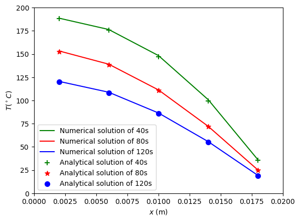
T_true_40 = analytical_solution(x, 40) # calculate the analytical solution
T_true_80 = analytical_solution(x, 80)
T_true_120 = analytical_solution(x, 120)
plt.figure()
plt.plot(x, output_explicit_dt_2[0], '-g', label='Numerical solution of 40s')
plt.plot(x, output_explicit_dt_2[1], '-r', label='Numerical solution of 80s')
plt.plot(x, output_explicit_dt_2[2], '-b', label='Numerical solution of 120s')
plt.scatter(x, T_true_40, s=50, c='g', marker='+', label='Analytical solution of 40s')
plt.scatter(x, T_true_80, s=50, c='r', marker='*', label='Analytical solution of 80s')
plt.scatter(x, T_true_120, s=50, c='b', marker='o', label='Analytical solution of 120s')
plt.xlabel('$x$ (m)')
plt.ylabel('$T$($^\circ C$)')
ax = plt.gca()
ax.set_xlim(0, 0.02)
ax.set_ylim(0, 200)
plt.legend(loc='lower left')
plt.show() # show the figure
# Investigate the effects of time step
dt = 8.0                                # time step size(dt<=08)
nx = 5                                  # number of spatial grid points
L = 0.02                                # length of the domain
dx = L / nx                             # spatial grid size
x = np.linspace(0.5*dx, L-0.5*dx, nx)   # spatial grid points
T0 = 200                                # initial temperature
rho_c = 1.0e7                           # fluid density plus specific heat
k = 10                                  # thermal conductivity
aW = k/dx
aE = k/dx
ap0 = rho_c * dx / dt
a = np.zeros((nx + 1, nx + 1))
b = np.zeros(nx + 1)
T = np.zeros(nx + 1)
T_old = np.zeros(nx + 1)
time = 0.0

for i in range(0, nx+1):
    T[i] = T0
    T_old[i] = T0

# Time loop
while time < 40:
    time += dt
    renew_explicit(a, b, nx)
    # TDMA(a, b, T, nx)
    Jacobi(a, b, T, nx)
    for i in range(1, nx+1):
        T_old[i] = T[i]
    output()

output_explicit_dt_8 = T[1:nx+1]
plt.figure()                            # create a new figure
plt.plot(x, output_explicit_dt_2[0], '-k', label='Numerical solution of 40s (dt=2)')
plt.plot(x, output_explicit_dt_8, '--k', label='Numerical solution of 40s (dt=8)')
plt.scatter(x, T_true_40, s=50, c='k', marker='+', label='Analytical solution of 40s')
plt.xlabel('$x$ (m)')
plt.ylabel('$T$($^\circ C$)')
ax = plt.gca()
ax.set_xlim(0, 0.02)
ax.set_ylim(0, 200)
plt.legend(loc='lower left')
plt.show()                              # show the figure
-----------
time = 8.0
200.0
200.0
200.0
200.0
0.0
-----------
time = 16.0
200.0
200.0
200.0
100.0
100.0
-----------
time = 24.0
200.0
200.0
150.0
150.0
0.0
-----------
time = 32.0
200.0
175.0
175.0
75.0
75.0
-----------
time = 40.0
187.5
187.5
125.0
125.0
0.0
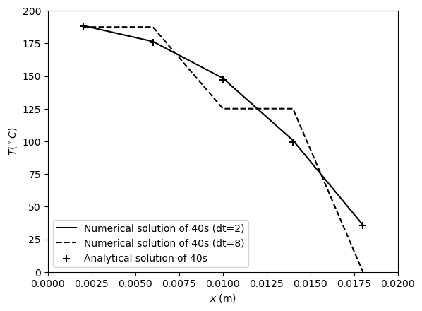
Note
Reducing the time step can effectively improve the accuracy of numerical calculation results.
Solve the equation by completely implicit method#
We can linearization the sourse term as $\(b = S_u + S_p T_p\)\( and take \)\(\theta = 0\)\( into the equation \)\(\begin{aligned} {{a_{P} T_{P}=}} & {{} {{} a_{W} \big[ \theta T_{W}+( 1 \!-\! \theta) \, T_{W}^{0} \big]+a_{E} \big[ \theta T_{E}+( 1 \!-\! \theta) \, T_{E}^{0} \big]+\big[ a_{P}^{0} \!-\! ( 1 \!-\! \theta) a_{W}-( 1 \!-\! \theta) a_{E} \big] T_{P}+b}} \\ \end{aligned} \)\( The discreted non steady-state advection equation by completely implicit method is \)\( a_{P} \, T_{P} \!=\! a_{W} T_{W} \!+\! a_{E} T_{E} \!+\! \, a_{P}^{0} \, T_{P}^{0} \!+\! S_{u} \)$ , where
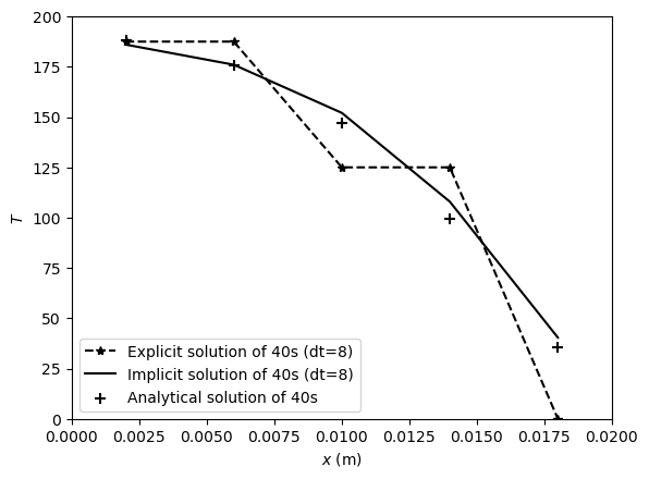
From the above equation, it can be seen that all coefficients maintain positive values So the fully implicit format is unconditionally stable for any time step At However, the calculation accuracy is only first-order intercept, and to ensure the calculation accuracy, a smaller time step should also be selected The fully implicit scheme is widely used in solving various non-stationary problems due to its unconditional stability and good convergence.
Here we go!
Internal Nodes 2, 3, 4
, where
Boundary Nodes 1 Take the bondary condition into the discreted equation like what we have done in explicit method, we will get $\(\rho c \Big( \frac{T_{P}-T_{P}^{0}} {\Delta t} \Big) \Delta x=\frac{k ( T_{E}^{0}-T_{P}^{0} )} {\Delta x} \)$
Boundary Nodes 5 $\(\rho c \Big( \frac{T_{P}-T_{P}^{0}} {\Delta t} \Big) \Delta x=\left[ \frac{k \left( T_{B}-T_{P}^{0} \right)} {\frac{\Delta x} {2}}-\frac{k \left( T_{P}^{0}-T_{W}^{0} \right)} {\Delta x} \right] \)$
Organize coefficient matrix By organizing the coefficient of above nodes, we can get
node |
\(a_{W}\) |
\(a_{E}\) |
\(a_{P}^{0}\) |
\(a_{P}\) |
\(S_{P}\) |
\(S_{u}\) |
|---|---|---|---|---|---|---|
1 |
0 |
\({\frac{k} {\Delta x}}\) |
\(\rho c {\frac {\Delta x}{\Delta t}}\) |
0 |
0 |
\(a_{w} + a_{E}+a_{P}^{0} -S_{P}\) |
2,3,4 |
\({\frac{k} {\Delta x}}\) |
\({\frac{k} {\Delta x}}\) |
\(\rho c {\frac {\Delta x}{\Delta t}}\) |
0 |
0 |
\(a_{w} + a_{E}+a_{P}^{0} -S_{P}\) |
5 |
\({\frac{k} {\Delta x}}\) |
0 |
\(\rho c {\frac {\Delta x}{\Delta t}}\) |
\(-{\frac{2k} {\Delta x}}\) |
\(-{\frac{2k} {\Delta x}}T_{B}\) |
\(a_{w} + a_{E}+a_{P}^{0} -S_{P}\) |
Solve algebraic equations (completely implicit method)#
What we need to do is just change the renew function.
# Update coefficients for implicit method
def renew_implicit(a, b, nx):
    a[1, 1] = ap0 + aE - 0
    a[1, 2] = -aE
    for i in range(2, nx):
        a[i][i - 1] = -aW
        a[i][i] = ap0 + (aW + aE - 0)
        a[i][i + 1] = -aE
    a[nx, nx - 1] = -aW
    a[nx, nx] = ap0 + aW + 2 * aW

    for i in range(1, nx + 1):
        b[i] = ap0 * T_old[i]
a = np.zeros((nx + 1, nx + 1))
b = np.zeros(nx + 1)
T = np.zeros(nx + 1)
T_old = np.zeros(nx + 1)
time = 0.0
dt = 8.0

for i in range(0, nx + 1):
    T[i] = T0
    T_old[i] = T0

# Time loop
while time < 40:
    time += dt
    renew_implicit(a, b, nx)
    # TDMA(a, b, T, nx)
    Jacobi(a, b, T, 100)
    for i in range(1, nx + 1):
        T_old[i] = T[i]
    output()

output_implicit_dt_8 = T[1:nx + 1]
-----------
time = 8.0
199.44751381215474
198.3425414364641
193.92265193370167
177.34806629834253
115.4696132596685
-----------
time = 16.0
197.85262965110962
194.66286132901928
184.11373279203934
153.9467659717347
76.97719849821435
-----------
time = 24.0
195.0190109483703
189.3517735428917
173.06236056515792
134.67020313366135
57.72492002601801
-----------
time = 32.0
191.00352102015404
182.97254116372153
162.18309654894873
119.63512390175754
47.01699279075872
-----------
time = 40.0
186.004571656615
176.00667292953688
152.07703773408934
107.93528490892314
40.39385409808811
# Visualization
plt.figure()                            # create a new figure
plt.plot(x, output_explicit_dt_8, '--*k', label='Explicit solution of 40s (dt=8)')
plt.plot(x, output_implicit_dt_8, '-k', label='Implicit solution of 40s (dt=8)')
plt.scatter(x, T_true_40, s=50, c='k', marker='+', label='Analytical solution of 40s')
plt.xlabel('$x$ (m)')
plt.ylabel(r'$T$')
ax = plt.gca()
ax.set_xlim(0, 0.02)
ax.set_ylim(0, 200)
plt.legend(loc='lower left')
plt.show()                              # show the figure
Exercise#
Can you solve the problem by using the Crank-Nicolson scheme?
Compare the results from the explicit, the Crank-Nicolson and the implict schemes regarding accuracy and stability.